Day 3 - Performing differential gene expression with nf-core/differentialabundance pipeline
Recap from Day 2
- Yesterday we covered:
- Outputs from Day 1 session (fetchngs pipeline)
- Inputs needed to run the rnaseq pipeline
- How to execute the rnaseq pipeline
Outputs from the rnaseq pipeline
- We should all have had an email from SCW HAWK - HPC SERVICES notifying you of a successful pipeline run.
- Sometimes the email function doesn’t work. We can just log in and check ourselves.
- To check, we need to log back onto HAWK, load the tmux module, and then open the session that we created.
Log on to HAWK
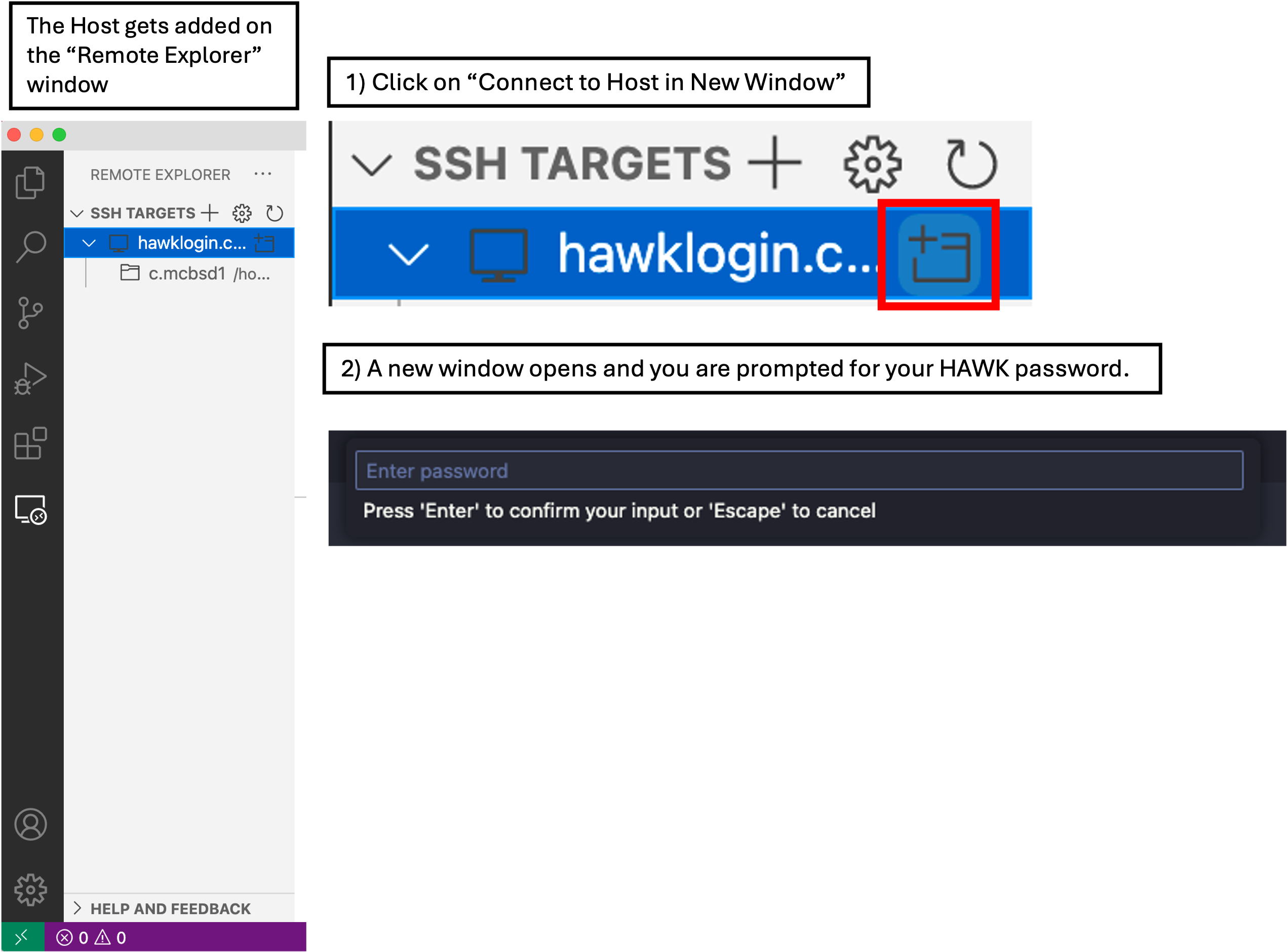
- In VSCode, click on the ‘Remote Explorer’ button, then click ‘Connect to Host in New Window’ button. This opens a new VSCode window with the remote host.
- You will be prompted (top box) to enter your password. Do this and hit enter.
- You are now connected to HAWK.
- Click on ‘Explorer’ and then ‘Open Folder’.
- A drop-down box appears at the top of the screen with a filepath. We need to change this to
/scratch/c.c1234567/rnaseq-courseand then click ‘OK’. - You may be prompted ‘Do you trust the authors this folder?’. Click ‘Trust all authors’ or ‘Yes’.
- You will now see that the directory will be open on the left of the window.
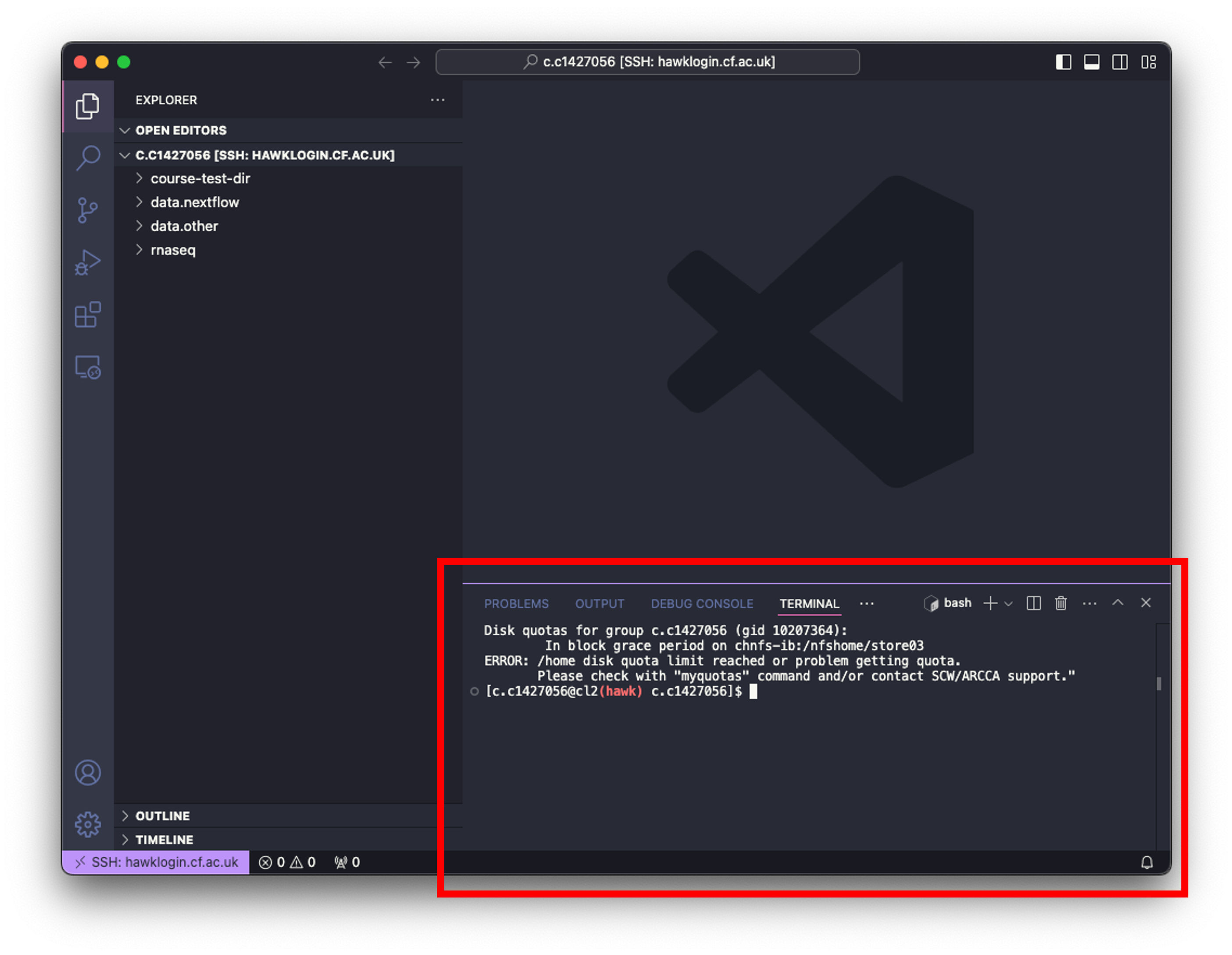
- Click on ‘Terminal’ at the top of your screen and select ‘New Terminal’.
- In the terminal window at the bottom of your screen, paste the following:
# log on to the cla1 node
ssh cla1

# move to the working directory (scratch)
cd /scratch/c.c1234567/rnaseq-course

# load tmux
module load tmux

# open our tmux session
tmux attach -t rnaseq
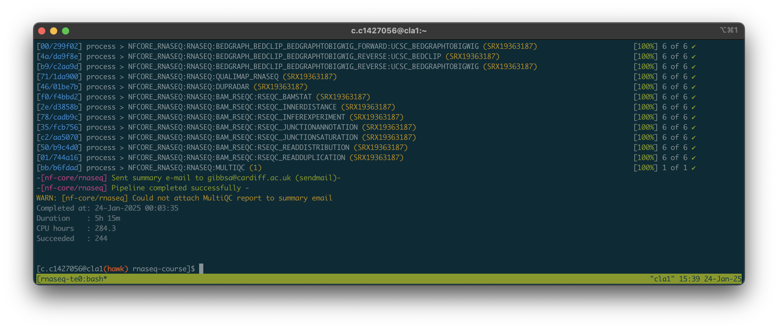
- Upon opening the session, we should have a window that looks like this:
Linux Users
#log onto HAWK
c.c1234567@hawklogin.cf.ac.uk
PASSWORD

# log on to the cla1 node
ssh cla1

#move to the working directory (scratch)
cd /scratch/c.c134567/rnaseq-course

#load tmux
module load tmux

#open our tmux session
tmux attach -t rnaseq
- The process took almost 6 hours. As all of us were using the pipeline at the same time, these times will likely vary. Download times will also depend on the size and number of files being downloaded.
- Some of you may have yours still running. Please let me know if this is the case and we can get you access to the outputs so you can continue.
Population of the output directory
- All of the outputs from the pipeline will have been placed into the output directory.
- We should have the following: fastqc, multiqc, pipeline_info, sortmerna, star_salmon, trimgalore.
pipeline_info directory
- This directory contains all the files relevant to the pipeline that was run, such as a nextflow report, pipeline report.
- These files can be used to make a report if needed (handy when writing methods section).
- We don’t need any of these files for the next stages.
sortmerna directory
- This directory contains the log files for each sample during the ribosomal RNA removal step.
- The log files contain information about the reads that matched the reference database(s).
- We do not need anything from this directory for the next stages.
trimgalore directory
- This directory contains the log files for each sample during the trimgalore step.
- Trimgalore tool is used to trim the adapter sequences from each sequencing file.
- The log files contain information about what sequencing adapters were removed from the samples etc.
- We don’t need any of these files for the next stages.
fastqc and multiqc directories
- One thing we need to check is the quality of the sequencing reads.
- The way we do this is to perform FastQC on each sample, which produces a report for each fastq file.
- As you can imagine, this can be a painstaking process if we were to check every file one by one.
- This is where MultiQC comes in handy - it produces one report for all of the FastQC results.
- It also takes the data from the other processing steps and feeds it into the report, giving us an overall rnaseq pipeline sequencing statistics report.
- We can view the report via the ‘Preview on Web Server’ extension. If anyone hasn’t installed this extension, please let me know so we can get you going.
Linux Users
- The MultiQC webpage report is located in `/scratch/c.c1234567/rnaseq-course/output/multiqc/star_salmon/’
- You will need to transfer the `multiqc_report.html’ file.
#move to a directory where you want to download the file to. I reccommend Downloads
cd Downloads

#transfer file from HAWK to the current directory. Make sure you include the dot (.)!
scp c.c1234567@hawklogin.cf.ac.uk:/scratch/c.c1234567/rnaseq/output/multiqc/star_salmon/multiqc_report.html .
Assessing the MultiQC report
- There is a great video that covers the outputs of the MultiQC report here.
- I won’t cover the whole report as there is too much to cover in one session.
- I will cover what I believe to be the most important parts, but please do have a good look through the whole report if you are interested.
- Using the ‘Explorer’ tab, navigate to following:
rnaseq-course/output/multiqc/star_salmon. - Right-click on
multiqc_report.htmlfile and click on ‘vscode-preview-server: Launch on browser’. - This will open the report on your default web browser.
STAR_SALMON DESeq2 sample similarity
- This section provides the user with a heatmap of sample-sample distances.
- It allows us to quickly check the similarity, and differences, between our samples.
- As we have the same condition between two different cell lines, we should expect there to be an obvious difference between them.
- As you can see, there is a high degree of similarity within the groups (as depicted by the red sections), and a low degree of similarity between the groups (as depicted by blue sections).
- If we were to analyse the whole dataset, which consists of 2 cell lines that have hypoxic and normoxic conditions (12 samples total, 6 samples per cell line, 3 samples per condition), we would expect a clear difference in similarities between the two cell lines, with only a slight difference in similarities between the conditions in the same cell line.
- We can use this plot to also quickly see if there are any potential outliers in our data.
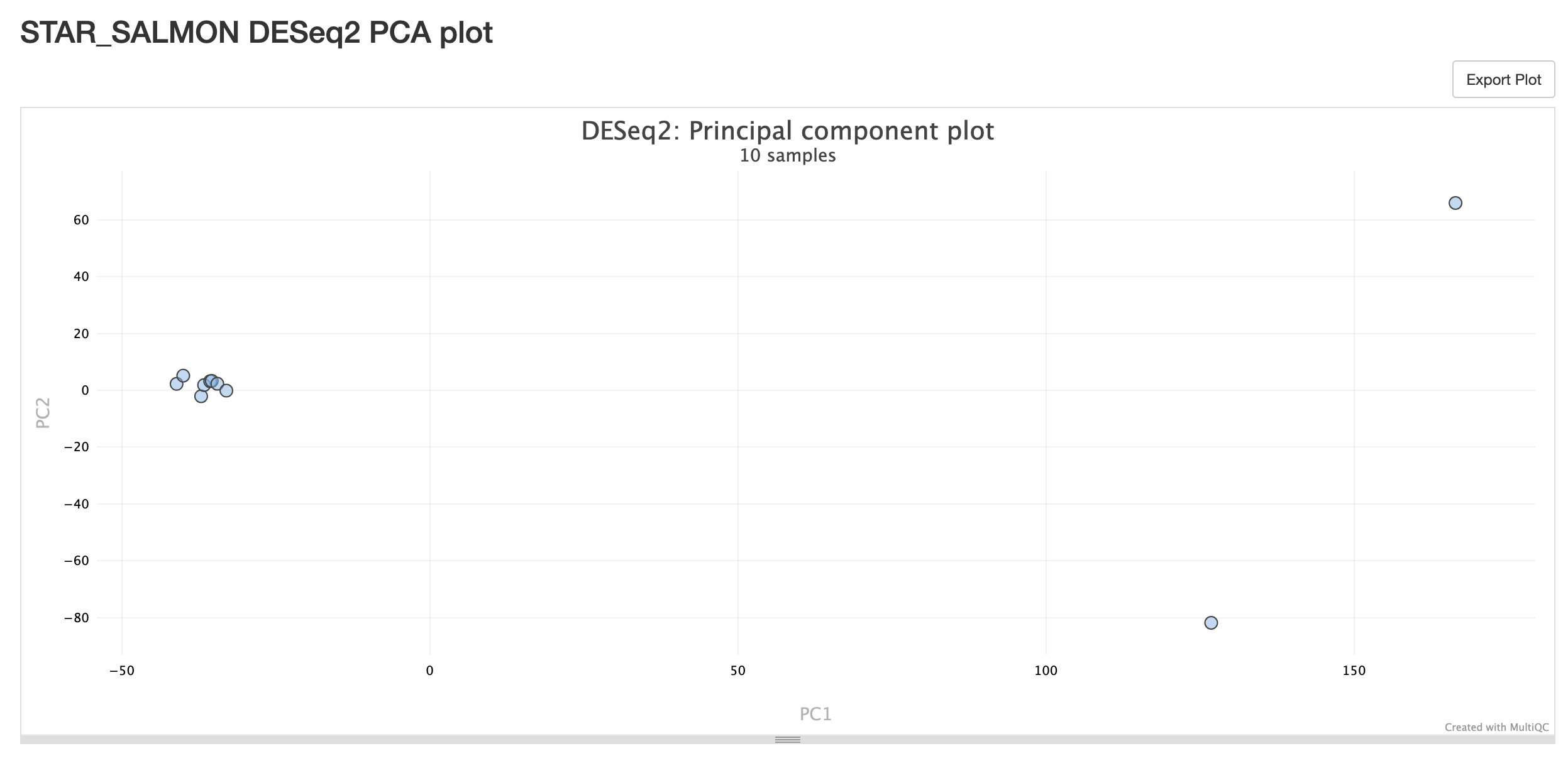
STAR_SALMON DESeq2 PCA Plot
- This Principal Component Analysis (PCA) plot is used to show us how similar or different each sample is to each other.
- PCA analysis is a method of simplifying multi-dimensional data.
- The analysis takes the gene expression data for each sample, which is a data table containing thousands of expression values for each gene, and represents this as one data point for each principle component.
- This data point represents the most variation in the dataset for the given principle component. The algorithm is then adjusted and reiterated to give another set of data points for the next principle component, and so on.
- This plot shows us the data points for principle component 1 vs principle component 2 (PC1 vs PC2).
- Don’t worry if you don’t quite get how the analysis works, here is a great video that nicely covers the method.
- All you need to know is that the closer the points are, the more similar the samples are. The more dispersed/further away the points are, the less similar the samples are.
- Here we can see that we have a nice cluster of points for one condition along both axes, indicating that we have a high degree of similarity between these 3 samples.
- We can also see on the left hand side, that for at least the PC1 axis, we have a hight degree of similarity for the other 3 samples. Not so much when we look at the PC2 axis.
- As we are only analysing the 2 groups and can see that there is a clear separation between them, this is as far as we need to go for this analysis.
- We will keep in mind, though, that we may have some outliers for the other sample group as they are more dispersed from each other.
QualiMap
Genomic origin of reads
- This tools is useful for giving us information about the mapped reads.
- As we have RNAseq samples, we would expect to get a lot of reads mapping to the exonic regions.
- In a good experiment, we would expect to get >80% of reads mapping to the exonic regions.
- I would say <60% reads mapping to the exonic regions would be a cause for concern.
FastQC Raw & Trimmed
- The pipeline performs FastQC on the raw reads and then on the trimmed reads.
- It is good practice to check both raw and trimmed fastQC results to ensure sample quality is improved or consistent after trimming.
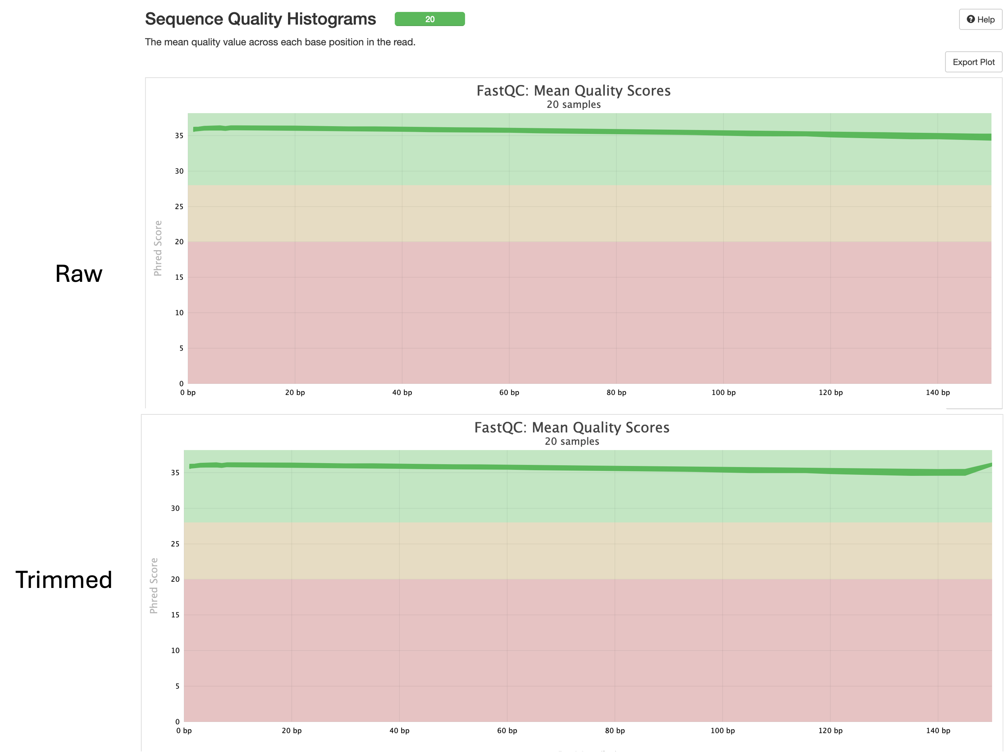
Sequence Quality Histograms
- This is the most handy output from the report.
- The tool generates a quality score for each sample and reports it as a histogram.
- What we are looking for is high quality scores across the length of the sequences.
- Here we can see that we have a mean score of 30 for all samples for both raw and trimmed.
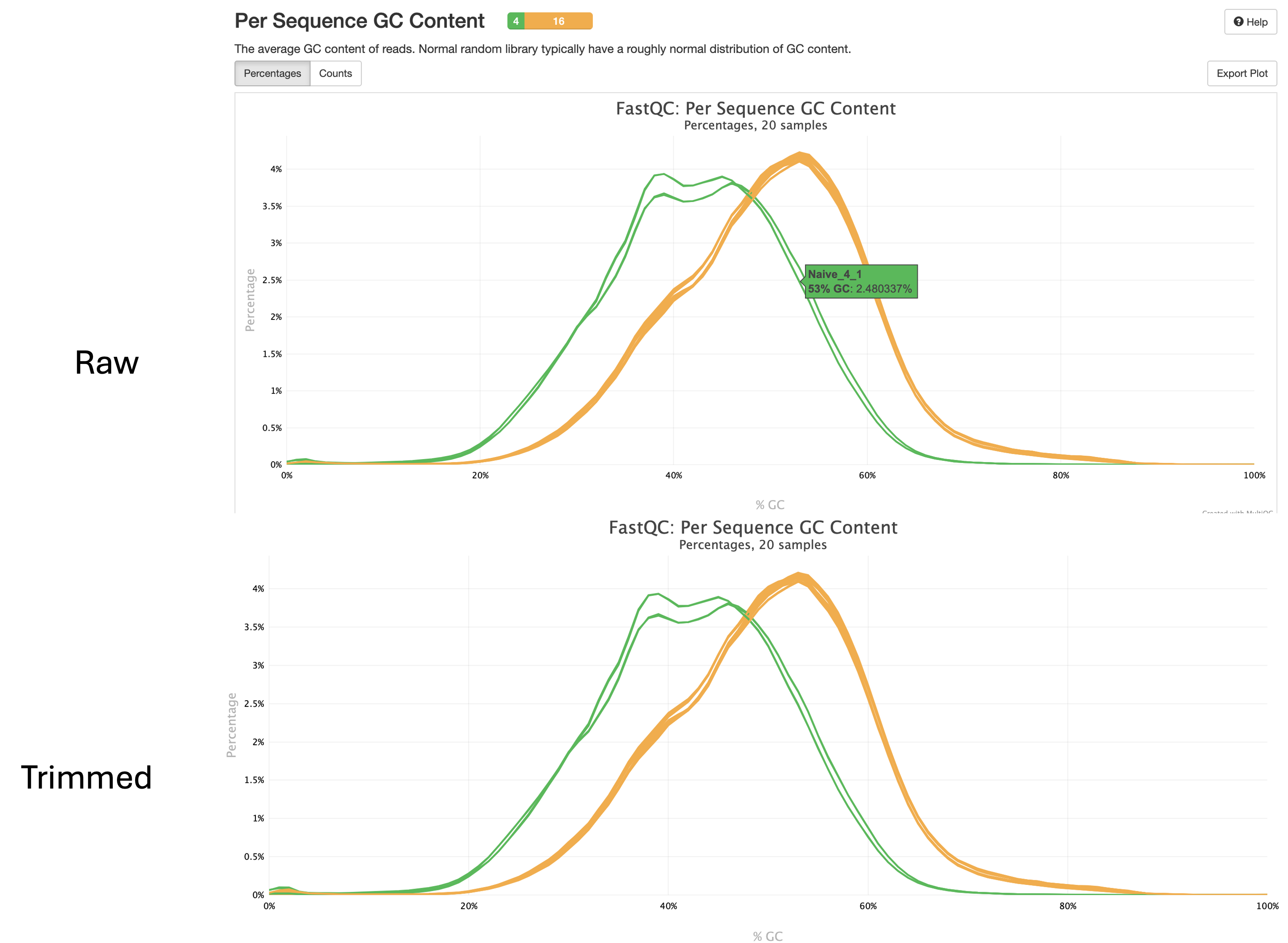
Per Sequence GC Content
- This plot shows us the average GC content of reads for each sample.
- We expect this value to be between 40% and 60% in humans and 40% and 50% in mice.
- Here we can see our GC content falls around 50% in this dataset for both raw and trimmed reads.
star_salmon directory
- This directory contains all of the main outputs for the pipeline.
- Here we will find the processed sample files as well as various other files such as files that contain the stats outputs from the various tools used during the pipeline. These files are used to generate the multiqc report that we just covered.
- I won’t go over each of these outputs here, but a full description of them can be found on the output section of the pipelines webpage.
- For those who don’t plan on running the differentialabundance pipeline (completely fine and up to you!), the files you may need to run your downstream differential analyses are:
SAMPLE/quant.genes.sf: Salmon gene-level quantification of the sample, including feature length, effective length, TPM, and number of reads.SAMPLE/quant.sf: Salmon transcript-level quantification of the sample, including feature length, effective length, TPM, and number of reads.
nf-core/differentialabundance pipeline
Required files:
resources/conditions.csv
- This file is not required by the pipeline, but is instead required by the script that I have written which runs the pipeline at the end.
- This file contains the sample ID’s and the corresponding condition information.
- To keep things less complicated and running smoothly, I have created this for you. If we needed to change this for another sequencing dataset though, we would right-click on the file and click on ‘Open With…’ then select the ‘CSV Editor’. This will open the file as a table, which will make it easier for you to edit.
- If you open the file by left-clicking, you will see that we are just using the cell line names as the condition information.
- When we run the pipeline, this file is merged with the first 4 columns from the
samplesheet.csvfile to create a new samplesheet that is needed for this pipeline to run.
resources/diff-abundance-samplesheet.csv
- This file is similar to the
samplesheet.csvfile that we used for the rnaseq pipeline, but differs in that it contains additional columns that contain information the pipeline needs to differentiate between sample groups etc. These columns are taken from theconditions.csvfile. - The column format is as follows to compare between the two groups:
| sample | fastq_1 | fastq_2 | strandedness | conditionOne |
|---|---|---|---|---|
| sampleA_1 | path/to/file | path/to/file | auto | GroupA |
| sampleA_2 | path/to/file | path/to/file | auto | GroupA |
| sampleA_3 | path/to/file | path/to/file | auto | GroupA |
| sampleB_1 | path/to/file | path/to/file | auto | GroupB |
| sampleB_2 | path/to/file | path/to/file | auto | GroupB |
| sampleB_3 | path/to/file | path/to/file | auto | GroupB |
- As we are running a truncated dataset for this course, we only have 2 conditions, GroupA and GroupB (HK-2 and 786-0). We will therefore only require one condition column.
- However, The whole dataset has 2 cell lines with 2 conditions. If we wanted to use the whole dataset and run different comparisons, we would need to add extra columns which group the samples accordingly.
See here how to add extra columns to perform extra comparisons
- If we wanted to compare firstly between the two cell lines regardless of conditions, we would use the `conditionOne` column and compare GroupA vs GroupB. - If we wanted to compare between the conditions, irrespective of the cell line, we would add a `conditionTwo` column and compare ConditionA vs ConditionB: sample|fastq_1|fastq_2|strandedness|conditionOne|conditionTwo |-----|-------|-------|------------|------------|-----------| sampleA_1|path/to/file|path/to/file|auto|GroupA|ConditionA sampleA_2|path/to/file|path/to/file|auto|GroupA|ConditionA sampleA_3|path/to/file|path/to/file|auto|GroupA|ConditionA sampleA_4|path/to/file|path/to/file|auto|GroupA|ConditionB sampleA_5|path/to/file|path/to/file|auto|GroupA|ConditionB sampleA_6|path/to/file|path/to/file|auto|GroupA|ConditionB sampleB_1|path/to/file|path/to/file|auto|GroupB|ConditionA sampleB_2|path/to/file|path/to/file|auto|GroupB|ConditionA sampleB_3|path/to/file|path/to/file|auto|GroupB|ConditionA sampleB_4|path/to/file|path/to/file|auto|GroupB|ConditionB sampleB_5|path/to/file|path/to/file|auto|GroupB|ConditionB sampleB_6|path/to/file|path/to/file|auto|GroupB|ConditionB - If we wanted to comapre the two conditions within the same samples, we would add a `conditionThree` column and compare GrpAConA vs GrpAConB and GrpBConA vs GrpBConB: sample|fastq_1|fastq_2|strandedness|conditionOne|conditionTwo|conditionThree |-----|-------|-------|------------|------------|------------|-------------| sampleA_1|path/to/file|path/to/file|auto|GroupA|ConditionA|GrpAConA sampleA_2|path/to/file|path/to/file|auto|GroupA|ConditionA|GrpAConA sampleA_3|path/to/file|path/to/file|auto|GroupA|ConditionA|GrpAConA sampleA_4|path/to/file|path/to/file|auto|GroupA|ConditionB|GrpAConB sampleA_5|path/to/file|path/to/file|auto|GroupA|ConditionB|GrpAConB sampleA_6|path/to/file|path/to/file|auto|GroupA|ConditionB|GrpAConB sampleB_1|path/to/file|path/to/file|auto|GroupB|ConditionA|GrpBConA sampleB_2|path/to/file|path/to/file|auto|GroupB|ConditionA|GrpBConA sampleB_3|path/to/file|path/to/file|auto|GroupB|ConditionA|GrpBConA sampleB_4|path/to/file|path/to/file|auto|GroupB|ConditionB|GrpBConB sampleB_5|path/to/file|path/to/file|auto|GroupB|ConditionB|GrpBConB sampleB_6|path/to/file|path/to/file|auto|GroupB|ConditionB|GrpBConB - Hopefully you can see how we can use these additional `condition` columns to compare different samples and groups etc.
- Again, to keep things as simple as possible, I have added some code into the
bin/differentialabundance.shscript which takes thesamplesheet.csvfile from the rnaseq pipe and theconditions.csvfile to make thediff-abundance-samplesheet.csvprior to executing the pipeline.
resources/contrasts.csv
- We will also need to provide a contrasts file that is used by the pipline to perform the differential gene expression analyses.
- This file tells the pipeline what columns to use for the testing, and which groups to compare in that column.
- The file contains 4 columns: id, variable, reference, target
- This file is already made and should be located in your
resourcesdirectory. If you click on it (or open it with the CSV Editor), it should look like this:
| id | variable | reference | target |
|---|---|---|---|
| 786-0_vs_HK-2 | conditionOne | HK-2 | 786-0 |
- Here,
idis used to give the analysis an id. This can be whatever you want. To keep things simple, we have kept with the cell line names. variablespecifies which column in thesamplesheet.csvfile the pipeline needs to look at to select samples for comparison. We have said to use theconditionOnecolumn.referencespecifies which group in theconditionOnecolumn is going to be the reference group. i.e. The group we are comparing against.targetspecifies the gorup in theconditionOnecolumn that will be used as the target group. i.e. The group that we use to compare.
resources/Homo_sapiens.GRCh38.110.gtf
- We also need to specify the human gene reference file which is used to annotate the genes during the analysis.
- We already have this file downloaded from the rnaseq pipeline.
resources/diff-abundance-params.yaml
- As with the other pipelines, we need a parameter file containing each option for the pipeline.
-
Again, we will need to edit it before we run.
-
We need to change the email address, and study name in this file (and the species if using a different one)
- Open the file in VSCode by simply clicking on it, then change your email address and scw account.
- Then save the file by clicking
File > Save. Close the file by clicking the ‘X’ next to the filename along the top of your window.
Linux Users
nano resources/diff-abundance-params.yaml

input: resources/diff-abundance-samplesheet.csv
outdir: output
-profile: rnaseq
matrix: output/star_salmon/salmon.merged.gene_counts.tsv
transcript_length_matrix: output/star_salmon/salmon.merged.gene_lengths.tsv
contrasts: resources/contrasts.csv
differential_min_fold_change: 2
gtf: resources/Homo_sapiens.GRCh38.110.gtf
email: <b>YOUR-EMAIL@cardiff.ac.uk</b>
study_name: <b>MY-STUDY-NAME</b>
study_type: rnaseq

#save and exit
ctrl + x
y
enter
- Note that we have included
study_nameandstudy_typein here, this is to make the outputs neater and is good practice. - In some cases, you may want to run the pipieline a few times with different comparisons etc, by changing the
study_nameparameter each time, we are ensuring a new directory is created isntead of overwriting the previous analysis.
resources/my.config
- We created this configuration file yesterday.
- We do not need to edit this file any further.
- Our scratch directory should now look like the following:
.
└── rnaseq/
    ├── bin/
    │   └── differentialabundance.sh
    ├── resources/
    │   ├── my.config
    │   ├── Homo_sapiens.GRCh38.110.gtf
    │   ├── *diff-abundance-samplesheet.csv* (This will be generated by the script)
    │   ├── diff-abundance-params.yaml
    │   ├── conditions.csv
    │   └── contrasts.csv
    ├── input/
    │   ├── fastq
    │   ├── metadata/
    │   ├── pipeline_info/
    │   └── samplesheet/
    └── output/
        ├── fastqc/
        ├── multiqc/
        ├── pipeline_info/
        ├── sortmerna/
        ├── star_salmon/
        │   ├── salmon.merged.gene_counts.tsv
        │   └── salmon.merged.gene_lengths.tsv
        └── trimgalore/
Executing the nf-core/differentialabundance pipeline
- Now that we have the files ready for the pipeline, we can go ahead and execute it.
- To run the pipeline, we need to be in the parent directory (rnaseq-course) directory.
- First of all, lets exit the rnaseq tmux session and create a new one for the rnaseq pipeline.
- In the terminal window at the bottom of your screen:
# detach from the fetchngs session
ctrl + b
d

# create new tmux session
tmux new -s diff-abundance

# load modules
module load nextflow/24.10.4
module load singularity/singularity-ce/3.11.4
- Now we can run the pipeline
# execute pipe
./bin/differentialabundance.sh

# leave pipeline running for a few minutes to ensure its working, then we can close the session:
crtl +b
d
- We will cover the outputs from this pipeline during the Day 3 session.